Data Lookup in Excel

2017-06-27

Hey all!

A boring-ish topic today, but its a basic one when it comes to excel and manipulating data.

There are four main ways of accessing data in another cell in excel.

1. Direct linking.

2. Vlookup & hlookup.

3. Sumproduct.

4. Index + match.

EXAMPLE SHEET

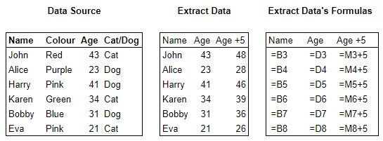
1. Direct linking

Direct linking is the simplest one where you enter = into a cell then click on the cell where you want to take the info from.

Formula:
={cell to be linked}

Pros:
– Simple.
– Fast (for small amounts).
Cons:
– Cannot adjust to the data changing.
– Impractical for large amounts of linking.

EXAMPLE

The methods below require you to know a piece of knowledge about what you want to look up, be it a name or uniqueID.

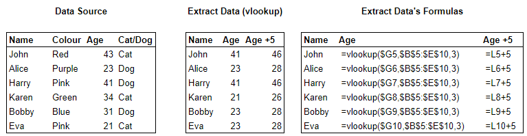
2. Vlookup & hlookup.

vlookup and hlookup work by taking a {key}, searching for it in the first row (hlookup) or column (vlookup) a {range}, it then returns a value that is {offset} from that where the searched col/row is 1 and the next one over/down is 2 etc.
What this means is that you must already know what you want to lookup based on something that you already have.

Formula:
– =vlookup({key},{region to be searched},{offset})
– =hlookup({key},{region to be searched},{offset})

Pros:
– It can adjust easily to data moving rows/cols.
– Faster than direct linking.
Cons:
– Can be a PITA to get done right, especially with large data-sets where you have to count the offset.
– Not as powerful as the following examples.

EXAMPLE

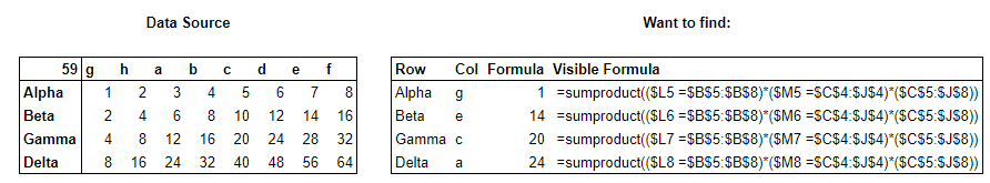
3. Sumproduct.

Sumproduct, is the most powerful formula on this list, but also the most complex, it is as if vlookup and hlookup had a child that was put on steroids.
This is also its very downfall.
Sumproduct searches a table like vlookup/hlookup but it is able to use multiple criteria to find what you want. To do this it can only return numerical values.
Sumproduct was not originally designed for looking up data it is a side effect on how excel processes TRUE and False statements, TRUE is 1 and FALSE is 0.
The formula turns everything in the lookup table to 0 except where the intersection of the two valid lookups is. (example on the spreadsheet to show this)

Formula:
– =sumproduct(({value to lookup 1}={header range to lookup 1})(({value to lookup 2}={header range to lookup 2})({table to lookup}))

Pros:
– Can look up multiple criteria
– Can deal with the data moving
Cons:
– Can only return numbers.
– As with vlookup setting the region makes it unable to addapt to more data than what is there.
– Large tables are calculation intensive.

EXAMPLE

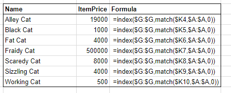
4. Index + match.

Finally the king and queen of data lookup, these are two separate formulas that when combined are able to efficiently pull data.
MATCH searches for something in a row/col and returns its position as a number, similar to the index above.
INDEX can take this number and return the value that is in that cell.
Of all the methods 2-4 it is the easiest as you specify what col/row to lookup a value you have and another to return the value you want.

Formula:
– =match({lookup value}, {lookup range},0) [the 0 is important here]
– =index({return range}, {index on range})
– =index({return range}, match({lookup value}, {lookup range},0))

Pros:
– Its fast.
– Light on calculations, important with a large spreadsheet.
– Easy to adjust.

Cons:
– Unable to select multiple criteria

EXAMPLE

I hope that was clear enough, if you have any questions don’t hesitate to ask. Either as a comment here or on my discord (see info page)